Getting Data In — ouRGeo Docs

01 Four ways in

However the data arrives, the import is R code you can keep.

Load Data files

Vector, raster, tabular and statistical files from disk. Jump to it.

Data Connector the web

14 web-API providers and open-data portals, with a visual query builder. Jump to it.

Create Data by hand

Build a data frame, matrix or vector from scratch. Jump to it.

.Rgeo big data

DuckDB-backed datasets for vector and raster too large for memory. Jump to it.

All four end the same way: the actual read is R code echoed to your console, so every import is reproducible and re-runnable without the GUI.

02 The Load Data dialog

Opened from the Load Data toolbar button. Pick a file and ouRGeo detects the format from its extension; you can override the guess. The form then shows only the settings that make sense for that format.

Supported formats

Group	Formats	Extensions
Delimited text	CSV, TSV, Text	`.csv` `.tsv` `.tab` `.txt`
Spreadsheets	Excel, ODS	`.xlsx` `.xls` `.ods`
Columnar / binary	Parquet, Feather, JSON	`.parquet` `.feather` `.json`
Statistical	SAS, SPSS, Stata	`.sas7bdat` `.sav` `.dta`
Vector spatial	Shapefile, GeoJSON, KML, and other OGR formats	`.shp` `.geojson` `.kml` `.kmz` `.gpkg` `.gml` `.dxf` `.gpx` `.fgb`
Raster	GeoTIFF and everything else GDAL reads	`.tif` `.tiff` `.img` `.vrt` `.asc` `.nc` `.jp2` `.grd` `.hgt` `.dem`

Common fields

File

The file to read. Reads No file selected until you pick one.

Format

Detected from the extension; override it when the extension lies.

Variable name

The R object the data lands in.

Detected columns

A preview of the columns found, with their inferred types. Types can be changed before loading — character, numeric, integer, logical, factor or Date — so you are not re-casting afterwards. Added columns lists any you define yourself.

Tabular settings

For CSV, TSV and text files.

Delimiter

Comma, Tab, Semicolon, Space, Pipe, or Custom for anything else.

Encoding

UTF-8, UTF-16, Latin-1 or Windows-1252 — the fix for mangled accented characters.

Header row

Whether the first row holds column names.

Skip rows

Number of leading rows to discard, for files with a preamble above the real header.

NA strings

Which literal values count as missing, e.g. NA, -9999, N/A.

Spreadsheet settings

Sheet

Which worksheet to read from a multi-sheet workbook.

Spatial settings

Layer

Which layer to read from a multi-layer container such as a GeoPackage.

CRS override

Assign a CRS when the file does not declare one. This labels the data — it does not move coordinates.

Reproject to

Transform into a different CRS on the way in. This does move coordinates.

Mixing these two up is the classic GIS mistake. Use CRS override when the data is in a known projection but carries no .prj; use Reproject to when the CRS is correct but you want the data in a different one.

Raster settings

Subdataset

For container formats such as NetCDF and HDF that hold several grids in one file.

Rasters are read with terra::rast() and arrive as a SpatRaster. They are read lazily — opening a very large GeoTIFF does not pull it into memory.

03 Creating data by hand

The Create data object button on the editor tab bar builds an R object from nothing — a data frame, matrix or vector. Define the columns and their types, enter values, and you get a normal R object plus the code that made it.

Useful for lookup tables, reclassification rules and small joins that would otherwise mean leaving the app to write a CSV.

04 The Data Connector

Browse the world’s public data catalogues without leaving the app — and get reproducible import code out the other end.

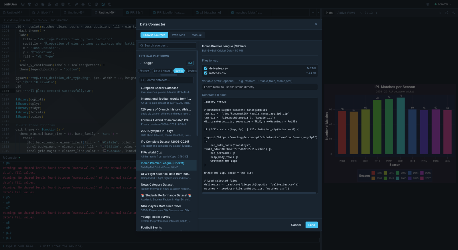
Opened from the Data Connector toolbar button. Three tabs across the top:

Browse Sources

A curated list of data sources. Below.

Web APIs

The provider framework — 14 API families with a shared query builder. Below.

Manual

Hand-entered URLs when you already know the endpoint. Below.

Only metadata and previews run in the interface. The actual import is generated R, echoed to your console and executed there — so your data pull is reproducible and survives without ouRGeo.

The Data Connector browsing a provider, building a query and previewing results. — The Data Connector — browse a provider, build a query, preview, and import as reproducible R.

05 Browse Sources

A catalogue of known data sources with their datasets. Pick a source, pick a dataset, and configure it. Until you do, the panel reads Select a source and dataset to configure it.

Files to load

Datasets distributed as file bundles list their contents here so you can choose what to import. If a bundle must be fetched before its contents are known, the panel reports Downloading dataset to inspect files…, and No files found if it turns out to be empty.

Variable name

The R object the import lands in.

Generated R code

The code that will run. Always shown before you commit.

Load

Runs the import in your session.

Sources marked LIVE are queried in real time rather than read from a cached catalogue.

Each dataset exposes only the arguments that are genuinely yours to choose — the ones that narrow the data rather than change what the dataset is. USGS NWIS is the worked example: daily values, water quality and groundwater are three different services, so there is no service picker, but the gauge and the measurement are fields, because a state of daily values is tens of thousands of rows a year and one gauge is a few hundred. Leave the site numbers empty and it falls back to the whole state; fill them in and they take over, because NWIS accepts exactly one of the two.

Every source and every provider carries a Help button that opens that API’s own documentation in your browser. A connector is a claim about somebody else’s service, and the questions it cannot answer — what a field means, why a portal is having a bad day — are answered there.

06 Web APIs

The most capable tab. Each provider is a family of servers speaking one API dialect; one shared interface drives all of them, so the workflow is the same everywhere:

Pick a provider, grouped by category.
Pick a server — the built-ins, or one you added yourself.
Cascade down to the resource you want. Depth varies by provider.
Build a query in the query builder: fields, operators, values.
Preview the result.
Load — the generated R runs and the object appears in your environment.

The providers

Category	Provider	What it gives you
Open Data	CKAN Portals	Datasets from any CKAN-powered open-data portal
Open Data	Socrata	Socrata portals, queried with SoQL
Geospatial	Esri ArcGIS REST	Feature and Map services as `sf`, with true curves preserved
	OGC API – Features	Modern OGC feature services
	WFS	Classic OGC Web Feature Services
	Macrostrat	Geology: stratigraphic columns, PBDB fossil collections, geologic map units, paleogeography (CC-BY 4.0)
Raster / Image Layers	Esri Image Services	Imagery and elevation, e.g. USGS 3DEP and USDA NAIP
	OGC WCS	Real coverage values via GetCoverage — EMODnet Bathymetry, DLR SRTM
	OGC WMS	Rendered RGB imagery via GetMap — NASA GIBS, terrestris
	STAC	SpatioTemporal Asset Catalogs: imagery assets, or item footprints as `sf`
	ERDDAP Grids	Gridded scientific data — NOAA CoastWatch, NOAA NCEI
Scientific	ERDDAP	Tabular scientific datasets
Statistics	SDMX	Statistical dataflows and series
Statistics	OData	OData services, queried with `$filter`

The query builder

One builder serves every provider; it serialises your query into whichever dialect the server speaks — SoQL, ArcGIS or CQL where, OData $filter, OGC and STAC parameters, ERDDAP constraints, SDMX keys.

Field list comes from the resource’s own metadata, marked for whether it is spatial and whether it is queryable.
Operators are whatever that provider actually supports, not a generic superset that fails at request time.
Value dropdowns are populated from the server’s distinct values where the API can supply them.
Lat/lng fill — when a resource has both a latitude and a longitude field, one click fills them from the map-view centre or the centre of any layer you already have.
Validation — some APIs reject invalid parameter combinations with a bare HTTP 500. Where that is known, the builder warns you and disables Load rather than letting you hit the error.

Large results

Before a big import the connector probes how much data is actually there. If the result is very large, or the server cannot deliver pages the size you asked for, a dialog asks how much you want. The wording adapts to the situation — SDMX, for instance, offers observations per series (1, 4, 12 or all) rather than a row count.

Adding your own servers

Every provider takes user-added servers. Paste the base URL of a CKAN portal, an ArcGIS REST endpoint or a WFS service and it joins the list, remembered between sessions.

07 Manual

For when you already have the URL. Enter it, set any query parameters and a response format, and ouRGeo generates the import code.

API URL

The endpoint to call.

Query parameters

Key/value pairs appended to the request.

Response format

How to parse what comes back, which decides whether you get an sf object or a data frame.

Start / End Date

Optional YYYY-MM-DD bounds for time-aware endpoints.

GeoTIFF / COG (URL)

Reads a remote Cloud-Optimized GeoTIFF in place via terra::rast("/vsicurl/…") — no download step.

08 Raster imports

The five raster providers share an export panel instead of a query builder, because you are choosing an extent and a resolution rather than filtering rows.

Extent

Current map view, or the dataset’s full extent.

Long-side pixel size

Output resolution, expressed as pixels along the longer axis.

Download size estimate

Updates as you change the above, so you find out before the request.

Time

Appears for time-aware services such as NASA GIBS.

Add to map when done

On by default. Registers the imported SpatRaster with the tile engine and zooms the map to it.

Large requests are chunked and mosaicked automatically — many servers return an error on their own advertised maximum size, so ouRGeo requests in slices of about 2048px and stitches the result with terra. Raster imports skip the tabular Data Viewer.

09 .Rgeo databases

DuckDB-backed storage for data that does not want to live in memory.

An .Rgeo file is a single-file database holding vector tables and rasters. You work with it through the Databases panel. Connecting a table gives you a lazy reference in R — a dplyr table proxy — rather than loading the rows.

Filtering happens in the database. dplyr verbs against a connected table are translated to SQL and run in DuckDB; only the result comes back.
Toolbox tools understand proxies. A tool that needs a real sf/data frame collects the proxy first, automatically, and the generated code shows it happening.
Rasters are stored as a tile pyramid — blocks with overview levels, written in strips so saving never holds the whole raster in RAM. Connecting one streams it back out into a GDAL-lazy SpatRaster.
Projects remember connections. Loading a .ourgeoproj reopens each .Rgeo and rebinds its table references, since restored proxies would otherwise point at a closed connection.

Requires DBI, duckdb and dplyr.

10 The R helper API

The functions the connectors generate — callable directly from your own scripts.

The Data Connector does not paste raw httr2 into your console. It calls named helper functions that ouRGeo defines in your R session, each of which handles the pagination, retry and format quirks of one API family. You can call them yourself — in a script, in a scheduled job, anywhere — with no GUI involved.

Function	Returns	What it handles for you
`ourgeo_read_arcgis()`	`sf`	Paginates EsriJSON and rebuilds Esri curves as true OGC `CIRCULARSTRING`/`COMPOUNDCURVE`/`CURVEPOLYGON` so arcs stay exact. Halves the page size and retries when a layer cannot satisfy its own advertised maximum.
`ourgeo_read_esri_image()`	SpatRaster	Chunked `/exportImage` requests, mosaicked with terra, with a retry per chunk.
`ourgeo_read_stac()`	`sf`	Treats STAC’s `limit` as the per-page cap it really is, follows pagination tokens, and halves the page size on a server error.
`ourgeo_read_stac_rasters()`	SpatRaster	Reads STAC item assets as rasters rather than footprints.
`ourgeo_read_wcs()`	SpatRaster	GetCoverage 2.0.1 for real data values. Reprojects the bbox, negotiates `SCALESIZE` axis naming across server implementations, and bisects the request when a server refuses the volume.
`ourgeo_read_wms()`	SpatRaster	Rendered RGB via GetMap 1.1.1 (which avoids the 1.3.0 axis-order trap), chunked, georeferenced locally and written to GeoTIFF.
`ourgeo_read_erddap_grid()`	SpatRaster	Imports griddap as `.esriAscii` for real float values, applies stride subsampling, and copes with descending latitude axes.
`ourgeo_read_sdmx()`	data frame	Fetches SDMX-CSV over `httr2` rather than base `url()`, avoiding TLS failures and short timeouts, and caps observations per series.
`ourgeo_read_odata()`	data frame	Generous timeout with retry, and `$top`/`$skip` pagination up to a record cap.

These exist because the obvious one-liner is usually wrong. sf::st_read() on an Esri query URL returns empty geometry; read.csv() on an SDMX URL fails with an SSL error on some systems. Each helper is the working version of an import that looks like it should be a single call.

Other functions worth knowing

ourgeo_linearize()

Converts curved geometry to straight segments. This is what the Linearize checkbox wraps your input in.

ourgeo_calc_crs()

Resolves the Auto-detect calculation CRS — the UTM zone for the data’s centroid, or identity for already-projected input.

11 Which R package powers what

ouRGeo only needs the packages for the features you actually use. If something is greyed out or errors on first use, this table is the place to look.

Packages	Needed for
`httpuv` `jsonlite` `later` `httr2`	Required. The R backend cannot start without these.
`sf`	All vector spatial work — import, geometry, the sf toolbox category
`terra`	All raster work — import, the 34 raster tools, tile serving
`geos`	The geos toolbox category
`dplyr`	Table, join, aggregate and type/string tools; `.Rgeo` proxies
`ggplot2` `ggspatial` `tidyterra`	ggplot2 map export and the chart builder
`tmap`	tmap map export
`maptiles`	Basemap tiles in exported maps
`png`	Encoding raster map tiles for the canvas
`sfarc`	Exact measurement and overlay on true curves — installs from Git, not CRAN (see below)
`DBI` `duckdb`	`.Rgeo` databases
`ggnewscale`	Only emitted by a ggplot2 raster export needing two fill scales at once

sfarc is the one package here that is not on CRAN yet. Install it from its Git repository:

install.packages("remotes")
remotes::install_github("CCurtis1988/sfarc")

It is pure R, so there is nothing to compile and Windows users do not need Rtools. Without it ouRGeo still starts — you just lose curved geometry entirely, and a layer containing CIRCULARSTRING or CURVEPOLYGON features will refuse to draw. See the install guide for the full setup.

The idiomatic API clients you might expect — RSocrata, esri2sf, rstac, rerddap, rsdmx — are not required. ouRGeo’s generated code uses httr2, jsonlite and sf::st_read directly, so there is nothing extra to install for the Data Connector.