oR
ouRGeo
Open-Source Spatial IDE
Home Features Docs Download Forum News Plugins Contribute Privacy Sign in Account Sign out

Maps, Drawing & Export

The map canvas end to end — styling layers, digitizing with snapping and true curves, and leaving with the R code that redraws it all.

01 The spatial editor

A GPU-accelerated map canvas that stays tied to your R objects.

Open it with the globe button in the toolbar. The map is MapLibre, so panning and zooming stay fluid over large vector data, and rasters are served as tiles by R itself rather than being flattened to a picture.

The important thing to understand: map layers are views onto R objects. A layer is not a copy of your data — it points at an object in your environment. Replace that object and the layer follows; delete it and the layer is invalidated.

Across the top of the panel is the ribbon. The Contents flyout holds your layer list. When you enter edit mode the ribbon is replaced by the geometry editing ribbon.

02 The map ribbon

Add Features
Opens the Add Features dialog — choose which spatial objects from your R environment to put on the map. Both vector layers and rasters are listed.
Selection tool
Toggles selection on and off. The button shows the active mode’s icon, and while it is active its tooltip says so. The chevron beside it opens Selection mode: Point Select (click features) or Lasso Select (drag a freehand shape). See Selection.
Change basemap
Opens the basemap picker.
Enter Edit Mode / Exit Edit Mode
Switches into digitizing. The ribbon is replaced by the geometry editing ribbon.
Unsaved edits
Appears while you have uncommitted geometry changes, listing what is pending. Use Save Edits to write them back to the R object.
Contents
Opens the layer list. See below.
Map Settings
A small menu with two toggles — Legend and North Arrow — each with its own settings button beside it. See Map decorations.
Export
Opens the export menu: Export to IMG, Export to Tmap, Export to ggplot. See Exporting a map.

03 Contents — the layer list

Your layers, topmost first. Empty, it reads No layers. Each row carries its own controls:

Layer name
The R object the layer is bound to. Click it to open the layer’s symbology.
Hide / Show
Toggles visibility without removing the layer.
Label settings
Opens the labelling dialog for that layer.
Remove
Takes the layer off the map. The R object is untouched — this removes the view, not the data.
Drag to reorder
Drag the handle to change draw order. The list order is the map order.
Unsaved edit badge
A count of pending geometry edits on that layer, with a reminder to use Save Edits.

04 Basemaps

The Change basemap button opens the provider picker. Several providers work with no configuration; those requiring an access token read it from Settings → Basemaps.

The basemap is more than decoration — when you export a map to ggplot2 or tmap, the chosen provider is carried into the generated code via maptiles, so the exported figure has the same backdrop as the screen.

05 Vector symbology

Click a layer in Contents to open its symbology. What you can set depends on the geometry type, but the structure is the same throughout: pick a single style for the whole layer, or drive the style from a column.

Column
Leave it unset for a single uniform style. Set it to drive colour from a column’s values — discrete values get categorical colours, continuous values get a ramp.
Fill / Border Color
Polygon interior and outline colour.
Border Thickness
Outline width in pixels.
Line Thickness
Stroke width for line layers.
Line Type
Solid or dashed patterns.
Shape
Marker shape for point layers.
Size
Marker size for point layers.
Halo Color / Halo Strength
A contrasting outline around symbols, which is what keeps points legible over a busy basemap.
Opacity
Layer transparency.

Colour ramps

Continuous colouring uses a named scale. The built-in set:

viridisplasma infernoblues redsgreens orangespurples RdYlGnRdBu pastel

06 Raster symbology

Raster layers get their own editor, opened the same way. Changes apply live — the tiles are re-rendered by R as you adjust, so you are looking at the real styling, not an approximation.

Render as
Single band, RGB composite, or categorical — the last for classified rasters such as land cover.
Stretch
How cell values map onto the colour range. Four options below.
Minimum – Maximum
Stretch across the band’s full observed range. Faithful, but one outlier flattens everything else.
Percent Clip
Discard a percentage from each tail before stretching. The usual choice for imagery.
Standard Deviations
Stretch to a number of standard deviations around the mean.
Custom Range
Type the minimum and maximum yourself — the way to make several rasters directly comparable.
Color ramp
The scales above, plus raster-only gray and terrain.
Resampling
How cells are interpolated when drawn away from native resolution.
Rendering
Per-band statistics and a histogram, sampled from the raster, so you can see the distribution you are stretching.
How raster display works. On adding a raster, R reprojects it to Web Mercator as a Cloud-Optimized GeoTIFF with internal overviews, then serves styled 256px PNG tiles to the canvas on demand. That is why a multi-gigabyte raster stays responsive, and why the first add of a large one takes a moment.

07 Labelling

Opened from the label button on a layer row. Grouped into sections:

Feature Labels
The master switch for labelling this layer.
Label Content
Which column supplies the text, and how it is composed.
Typography
Font — Noto Sans, Open Sans or Arial Unicode MS — plus size and weight.
Text Style
Colour, Outline (a halo that keeps text readable over imagery), and Transform for upper/lower casing.
Placement
Where labels sit relative to their feature, with Anchor controlling which part of the text box is pinned to that point.
Conflict Resolution
What happens when labels collide — whether to hide the loser or allow overlap.
Visibility
Zoom range over which labels are drawn, so a dense layer only labels once you are close enough.

08 Legend, north arrow and scale bar

The Map Settings menu on the ribbon toggles the Legend and North Arrow, each with a settings button for its own dialog.

Legend
Built from your layers’ symbology. Its dialog controls which layers appear, titles, and position.
North Arrow
Style, size and placement.

These are not only screen decoration. Title, subtitle, caption, legend, north arrow, scale bar, graticules and panel border are all carried into exported map code, where they become real ggplot2 or tmap elements rather than being redrawn by hand.

09 Selection and identify

Selecting

Activate the selection tool on the ribbon and pick a mode:

Point Select
Click features one at a time.
Lasso Select
Drag a freehand shape; everything inside is selected.

A selection is more than a highlight — it becomes a scope. Toolbox tools offer Use only current view, which restricts the operation to the selected features and shows the slicing in the generated code.

Identify

Clicking a feature brings up its attributes in a popup. For newly drawn features, the attribute popup can be made to appear automatically — see Settings → Spatial Editor → Drawing → Attribute popup for new features.

Query by attribute

Selection is not limited to clicking. A selection query dialog builds an attribute expression to select by — the map equivalent of the toolbox’s condition builder.

10 Drawing and geometry editing

Digitizing built to CAD conventions — snapping, typed coordinates, true curves.

Enter Edit Mode swaps the ribbon for the geometry editing ribbon. Until you pick a feature it prompts Edit Mode — click a feature on the map.

Modes

Create
Start a new feature.
Draw
Add geometry to the feature in progress.
Select
Pick an existing feature to work on.
Modify
Change existing geometry.
Edit Vertices
Move, add and delete individual vertices.
Move Feature
Translate a whole feature without reshaping it.

Segment and shape tools

The Choose tool control picks what the next click lays down. Segment type switches between straight and curve construction.

ToolWhat it draws
Straight LineAn ordinary straight segment.
Arc SegmentA true circular arc through control points.
Endpoint ArcAn arc defined by its endpoints.
Tangent CurveA curve continuing tangentially from the previous segment — the road-alignment case.
Bézier CurveA Bézier through control points.
CircleA complete circle.
RectangleAn axis-aligned rectangle.
FreehandFollows the cursor as you drag.
TraceFollows the boundary of an existing feature — how you get coincident borders with no gaps or slivers.
OffsetA parallel copy at a set perpendicular distance in metres. Negative values offset the other way.
Add Point(s)Point features — each click appends a row.
Distance & Bearing BType each course instead of clicking — see below.
Curve UThe same strip, starting on a curved course: tangent curve, curve, spiral, spiral–curve–spiral or free curve.
Arc, endpoint-arc and tangent-curve segments produce true curved geometry — CIRCULARSTRING and friends — not a polyline approximation. That is what lets sfarc measure them exactly later.

Snapping

Toggle snapping turns it on and off; Snapping options opens the Snap to list. Snapping works across every visible layer and the shape you are currently drawing, backed by a spatial index so it stays instant over dense data.

VerticesEdges MidpointsIntersections

Priority runs vertex > intersection > midpoint > edge, so the most meaningful target wins when several are in range.

Precise input — Distance & Bearing

An entry box in the ribbon takes typed coordinates instead of clicks, in the format lng,lat · d100 a45:

# Absolute coordinate
-122.42, 37.77

# Relative: 150 m at 45° clockwise from north, from the last vertex
d150 a45

For a whole traverse there is a tool of its own. Distance & Bearing (B) opens a docked strip: say where you are measuring from, then enter each course in the notation your notes are already written in.

Bearing notations
Azimuth, degrees-minutes-seconds, quadrant bearing (N45°30′E), deflection from the last course (L/R) and angle right. An entry that can only mean one thing is taken to mean it — N45°30′E typed while the notation says Azimuth is read as a quadrant bearing rather than refused.
Distance units
Metres, feet, US survey feet (the unit of most State Plane zones, and 2 ppm from the international foot), chains and miles — or type 150ft and the unit comes with the number.
Geodesic or grid
Geodesic distances use Vincenty’s method on the WGS 84 ellipsoid, not a sphere. But a bearing off a plat in a projected CRS is measured from grid north and its distance is a grid distance, so a projected layer defaults to its own grid in its own unit, and the strip always names which basis is in force. Measuring a grid traverse geodesically rotates the whole figure by the grid convergence — up to 3° at a UTM zone edge — and it still closes, so nothing on screen would tell you.
Curved courses U
Five kinds: tangent curve, curve, spiral, spiral–curve–spiral and free curve. Give any two of radius, arc length, chord, tangent, external, mid-ordinate, central angle or degree of curve; the strip prints all of them back, which is how a curve is checked against the plat that quotes them redundantly. A pair that fits two perfectly ordinary curves is refused by name with both angles listed rather than guessed at.
On a point layer
You place a reference point to measure from — a temporary mark, not a row in your data — and each course fills the row you are on and moves to the next, exactly as clicking does. Click elsewhere to re-place it, which flushes the run first, because the traverse it describes has just been broken.
Closure
Once a figure could close, the strip reports how far it is from closing and the 1:N a surveyor judges it by. A curve contributes its arc, never its chord.
Finishing a traverse echoes a runnable ourgeo_traverse() call naming the origin, the courses and the CRS. The geometry ouRGeo writes records coordinates; the distances and bearings they came from would otherwise be lost, and that call is what keeps them.

Finishing and undoing
Commit geometry Enter or double-click
Finishes the feature and advances to the next row.
Add a new row and keep drawing Enter
Commits and immediately starts another feature.
Save current part, start the next N
For multi-part geometry.
Start a hole in the polygon H
Begins an interior ring.
Remove last vertex Backspace
Steps back one point.
Undo / Redo Ctrl+Z / Ctrl+Y
Undo works through draft edits first, then staged commits.
Finish the session Esc
Closes the drawing session.
Leave edit mode
Returns to the normal map ribbon.
Drawn edits are staged, not written straight through. Use Save Edits to commit them back to the R object — until you do, the ribbon shows an unsaved-edit count and the affected layers are flagged in Contents.
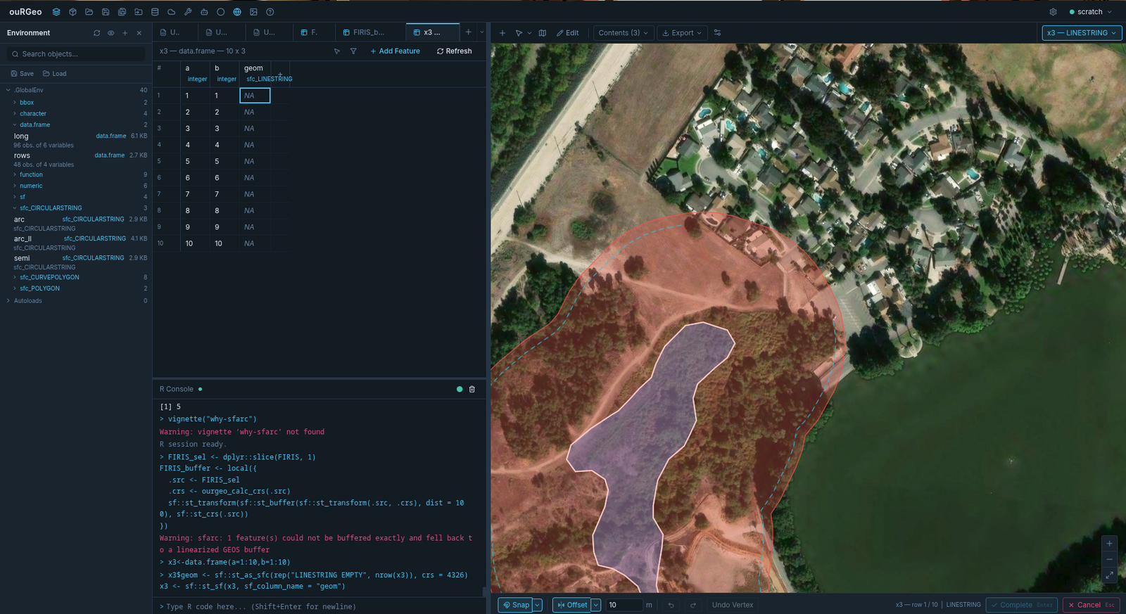
Snapping to an intersection while entering a precise distance-and-bearing vertex.
Snapping to an intersection while entering a precise distance-and-bearing vertex — CAD-grade digitizing.

11 Exporting a map

The Export menu on the ribbon has three destinations.

Export to IMG

Renders the map to an image file. Choose Format, Size, Directory and File, then Export. The map is re-rendered at the size you ask for rather than screenshotted, so the output is publication resolution.

Export to ggplot / Export to Tmap

The interesting ones: instead of an image, you get the R code that draws your map.

ouRGeo reads your on-screen map — layers, symbology, labels, legend, north arrow, scale bar, graticules, titles — and generates complete, standalone ggplot2 or tmap code that reproduces it. Run it, edit it, put it in a paper’s supplementary material, drop it into an R Markdown document.

  • Vector layers become the matching geoms with your fills, colours, widths and scales.
  • Raster layers keep their on-map symbology — geom_spatraster with a matching scale_fill_gradientn(), or geom_spatraster_rgb() for RGB composites; tm_raster with the equivalent tmap scale.
  • Basemaps are emitted via maptiles.
  • Annotations — title, subtitle, caption, legend, north arrow, scale bar, graticules and panel border — are written as real elements, and can be overridden in the dialog before generating.
This closes the loop that the rest of ouRGeo opens. You style a map by clicking, and leave with the script that makes it — so the figure can be regenerated when the data changes, by someone who never opens the app.