01 What the Toolbox is
87 point-and-click geoprocessing tools across seven categories — and every one of them writes R code you can keep.
Open the Toolbox from the Toolbox button in the top toolbar. Pick a tool, fill in the form, and press Run. The result lands in your R environment as a new object and opens in the Data Viewer.
What makes this different from a normal GIS toolbox is the Code Preview pane at the bottom of every tool form. It shows the exact R that your form settings produce, live, as you type. Running the tool runs precisely that code in your session — there is no hidden step, and nothing happens that you can’t see, copy, or edit.
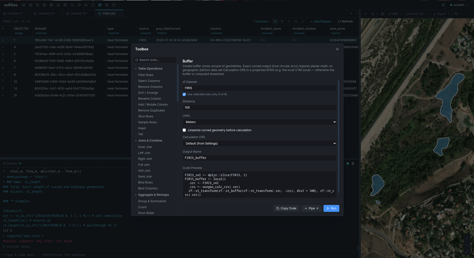
02 The Toolbox dialog
The dialog is split down the middle: a searchable tool tree on the left, and the selected tool’s form on the right.
03 The tool form
Every tool form is generated from the tool’s own definition, so they all behave the same way. Fields appear top to bottom, the code preview sits underneath, and the action buttons are pinned to the bottom-right.
Code Preview
The R your settings currently produce. It updates on every keystroke and never lags behind the form. This is the single most useful part of the Toolbox: it is how you learn the R equivalent of a GUI operation you already know.
Use only current view
When a dataset has an active selection or the map is zoomed to a subset, this checkbox restricts the tool to those features rather than the whole layer. The generated code slices the dataset first, so the restriction is visible in the preview like everything else.
Buttons
|> chain. See
Piping tools together. Disabled until a dataset is chosen.04 Field types
The parameter columns in the reference tables below use these field types.
parcels in Buffer
suggests parcels_buffered — and you can overwrite it. Reusing an
existing name overwrites that object.The condition builder
Filter Rows builds compound conditions without you writing the expression. Press Add Condition for each clause and join clauses with AND or OR. The right-hand side can be a literal value (val) or another column (col).
| Group | Operators |
|---|---|
| Comparison | == equal to, != not equal to,
> greater than, >= greater or equal,
< less than, <= less or equal |
| Membership | %in% in set — enter a comma-separated list |
| NA / Special | is.na, !is.na,
is.null, !is.null, is.nan,
is.finite, is.infinite |
| String / Pattern | grepl (regex),
grepl (ignore case), startsWith, endsWith,
nchar > (length greater than N) |
05 Linearize and Calculation CRS
Two options that only appear on spatial tools, and that decide whether your curved geometry survives the operation.
Linearize curved geometry before calculation
Every tool in Spatial — sf and Spatial — geos carries this checkbox — the one exception is Points from XY Columns, which has no geometry to linearize. It is off by default, and off is what you usually want.
- Unticked — curved geometry (
CIRCULARSTRING,COMPOUNDCURVE,CURVEPOLYGON) is passed through as-is, sosfarccan compute on the true arc and return an exact answer. - Ticked — the input is chopped into straight segments first by wrapping
it in
ourgeo_linearize(). You lose exactness, but you gain access to operations GEOS can only perform on polylines.
Calculation CRS
Exact curved maths is planar. On geographic (lat/lon) data an arc has no constant radius, so nine tools — Buffer, Intersection, Union (both), Difference, Erase, Clip, Centroid and Simplify — add a Calculation CRS dropdown. The generated code projects into that CRS, computes, and projects the result back to the layer’s own CRS, so what you get out is still in the coordinate system you started in.
ourgeo_calc_crs(): picks the
UTM zone from the dataset’s centroid for geographic input, and does nothing
for input that is already projected.32610.Raster tools have neither option. Linearize and Calculation CRS are sf/geos concepts;
terra handles reprojection explicitly through
Reproject Raster.
06 Piping tools together
Pressing Pipe → instead of Run chains tools into one R pipeline rather than creating an intermediate object per step. Configure a tool, press Pipe →, pick the next tool, and repeat; press Run on the last one to execute the whole chain at once.
The result is a single readable expression:
# Filter, then buffer, then dissolve — one pipeline, one output object
sites_final <- sites |>
  dplyr::filter(status == "active") |>
  sf::st_buffer(units::set_units(250, m)) |>
  sf::st_union()
- The output name is locked from the first step — the chain produces one object, not one per tool.
- Column dropdowns in later steps show the columns that will exist at that point, predicted from the earlier steps. Renaming, selecting or mutating a column in step one is reflected in step two’s dropdown without R having run yet.
- The banner across the top of the form traces the chain as you build it.
- Clear pipeline (the × on the banner) abandons the chain.
07 Tool reference
All 87 tools, by category.
The Parameters column lists each tool’s inputs in the order the form
shows them; the output-name field is on every tool and is omitted here. The
R call column names the main function the tool generates — useful when
you want to look something up with ? in the console.
Linearize and
Calc CRS
mark the tools that carry those extra options, described in
section 05.
Filtering is optional — with the box empty every tool stays in the page, so your browser’s own find (Ctrl + F) searches all of them.
08 Table Operations 11 tools
Row- and column-level work on any dataset — tabular or spatial. Every tool here emits dplyr, so an sf layer keeps its geometry column throughout.
| Tool | What it does | Parameters | R call |
|---|---|---|---|
| Filter Rows | Keep rows matching one or more conditions. | Dataset (any dataset) Conditions |
dplyr::filter() |
| Select Columns | Keep only the specified columns. | Dataset (any dataset) Columns to Keep (columns) |
dplyr::select() |
| Remove Columns | Drop the specified columns. | Dataset (any dataset) Columns to Remove (columns) |
dplyr::select() |
| Sort / Arrange | Sort rows by one or more columns, each ascending or descending. | Dataset (any dataset) Sort Columns |
dplyr::arrange()dplyr::desc() |
| Rename Column | Rename one column to a new name. | Dataset (any dataset) Column to Rename (column) New Name |
dplyr::rename() |
| Add / Mutate Column | Create a new column using an R expression. | Dataset (any dataset) New Column Name Expression |
dplyr::mutate() |
| Remove Duplicates | Remove duplicate rows, optionally based on specific columns. | Dataset (any dataset) Key Columns (optional) (columns) |
dplyr::distinct() |
| Slice Rows | Select rows by position (from–to, 1-based). | Dataset (any dataset) From Row (default 1) To Row (default 10) |
dplyr::slice() |
| Sample Rows | Randomly sample rows by count or fraction. | Dataset (any dataset) Sample Type (Count (n), Fraction (0–1)) Value (default 100) |
— |
| Head | Return the first n rows. | Dataset (any dataset) Rows (n) (default 6) |
— |
| Tail | Return the last n rows. | Dataset (any dataset) Rows (n) (default 6) |
— |
09 Joins & Combine 2 tools
Stack or splice two datasets together. For joining by location rather than by value, see Spatial — sf’s Spatial Join.
| Tool | What it does | Parameters | R call |
|---|---|---|---|
| Bind Rows | Stack two datasets vertically (same columns). | Dataset 1 (any dataset) Dataset 2 (any dataset) |
dplyr::bind_rows() |
| Bind Columns | Merge two datasets side by side (same number of rows). | Dataset 1 (any dataset) Dataset 2 (any dataset) |
dplyr::bind_cols() |
10 Aggregate & Reshape 5 tools
Collapse many rows into summary rows, and pivot between long and wide layouts.
| Tool | What it does | Parameters | R call |
|---|---|---|---|
| Group & Summarize | Group rows by a column and compute an aggregate statistic. | Dataset (any dataset) Group By Column (column) Aggregate Column (column) Function (Sum, Mean, Count (n), Min…) Result Column Name |
dplyr::n()dplyr::group_by() dplyr::summarize() |
| Count | Count the number of rows per group. | Dataset (any dataset) Column (column) |
dplyr::count() |
| Pivot Wider | Spread rows into columns (long → wide format). | Dataset (any dataset) Names From Column (column) Values From Column (column) |
tidyr::pivot_wider() |
| Pivot Longer | Gather columns into rows (wide → long format). | Dataset (any dataset) Columns to Pivot (columns) Names To Values To |
tidyr::pivot_longer() |
| Frequency Table | Compute a frequency table for a column. | Dataset (any dataset) Column (column) |
— |
11 Type & String 8 tools
Fix the things that are wrong with data as it arrives — wrong column types, padded whitespace, NAs, values that need splitting out of one field.
| Tool | What it does | Parameters | R call |
|---|---|---|---|
| Cast Column Type | Convert a column to a different data type. | Dataset (any dataset) Column (column) Target Type (Character (text), Numeric, Integer, Logical…) |
dplyr::mutate() |
| String Replace | Replace a pattern in a text column. | Dataset (any dataset) Column (column) Pattern Replacement |
dplyr::mutate() |
| To Upper / Lower | Convert a text column to upper or lower case. | Dataset (any dataset) Column (column) Direction (UPPER CASE, lower case) |
dplyr::mutate() |
| Trim Whitespace | Remove leading/trailing whitespace from a text column. | Dataset (any dataset) Column (column) Which Side (Both, Left only, Right only) |
dplyr::mutate() |
| Fill NA Values | Replace NA values in a column with a specified value. | Dataset (any dataset) Column (column) Fill Value |
tidyr::replace_na() |
| Coalesce Columns | Combine two columns, using the second as a fallback for NAs. | Dataset (any dataset) Primary Column (column) Fallback Column (column) New Column Name |
dplyr::mutate()dplyr::coalesce() |
| Filter by Pattern | Keep rows where a text column matches a pattern (regex). | Dataset (any dataset) Column (column) Pattern (regex) |
dplyr::filter()stringr::str_detect() |
| Separate Column | Split one column into multiple columns by a separator. | Dataset (any dataset) Column to Split (column) New Column Names (comma separated) Separator |
tidyr::separate() |
12 Spatial — sf 16 tools
Geometry operations through the sf package. These are the tools that understand curves: leave Linearize unticked and a CIRCULARSTRING stays exact.
| Tool | What it does | Parameters | R call |
|---|---|---|---|
| Buffer | Create buffer zones around sf geometries. Exact curved output (true circular arcs) requires planar math: on geographic (lat/lon) data set Calculation CRS to a projected EPSG (e.g. the local UTM zone) — otherwise the buffer is computed linearized. LinearizeCalc CRS |
sf Dataset (sf layer) Distance (default 100) Units (Meters, Kilometers, Feet, Miles) Segments per Quadrant (default 30; shown when relevant) |
units::set_units()sf::st_buffer() |
| Intersection | Return the shared area between two sf layers. LinearizeCalc CRS |
sf Dataset 1 (sf layer) sf Dataset 2 (sf layer) |
sf::st_intersection() |
| Union (Dissolve) | Dissolve all features in an sf layer into a single geometry. LinearizeCalc CRS |
sf Dataset (sf layer) | sf::st_union() |
| Union (Merge Two Layers) | Combine two sf layers and dissolve all features. LinearizeCalc CRS |
sf Dataset 1 (sf layer) sf Dataset 2 (sf layer) |
sf::st_union()dplyr::bind_rows() |
| Difference | Return the part of Dataset 1 that falls outside Dataset 2. LinearizeCalc CRS |
Target sf Dataset (sf layer) Clip sf Dataset (sf layer) |
sf::st_difference() |
| Erase | Erase the area of Dataset 2 from Dataset 1 (using unioned erase layer). LinearizeCalc CRS |
Target sf Dataset (sf layer) Erase sf Dataset (sf layer) |
sf::st_difference()sf::st_union() |
| Clip | Clip features to the extent/shape of a second sf layer. LinearizeCalc CRS |
Target sf Dataset (sf layer) Clip sf Dataset (sf layer) |
sf::st_intersection()sf::st_union() |
| Spatial Filter | Select features that satisfy a spatial predicate with another layer. Predicates are GEOS-only — tick Linearize for curved inputs. Linearize |
Features sf Dataset (sf layer) Filter by sf Dataset (sf layer) Predicate (Intersects, Within, Contains, Overlaps…) |
sf::st_filter() |
| Spatial Join | Join attributes from a second layer based on spatial relationship. Spatial joins are GEOS-only — tick Linearize for curved inputs. Linearize |
Left sf Dataset (sf layer) Right sf Dataset (sf layer) Join Type (Left Join, Inner Join) |
sf::st_join() |
| Centroid | Compute centroids of sf geometries. LinearizeCalc CRS |
sf Dataset (sf layer) | sf::st_centroid() |
| Add Area Column | Add a column containing the area of each feature. Linearize |
sf Dataset (sf layer) New Column Name |
dplyr::mutate()sf::st_area() |
| Add Length Column | Add a column containing the length of each line feature. Linearize |
sf Line Dataset (sf layer) New Column Name |
dplyr::mutate() |
| CRS Transform | Reproject an sf object to a different coordinate reference system. Linearize |
sf Dataset (sf layer) Target CRS (EPSG or proj string) |
sf::st_transform() |
| Simplify | Simplify geometries by removing vertices below a tolerance. GEOS-only — tick Linearize for curved inputs. LinearizeCalc CRS |
sf Dataset (sf layer) Tolerance (dTolerance) (default 100) Preserve Topology (Yes (recommended), No) |
sf::st_simplify() |
| Cast Geometry | Convert geometry type (e.g. POLYGON → MULTIPOLYGON). GEOS-only — tick Linearize for curved inputs. Linearize |
sf Dataset (sf layer) Target Geometry Type (POINT, MULTIPOINT, LINESTRING, MULTILINESTRING…) |
sf::st_cast() |
| Points from XY Columns | Convert a tabular dataset with coordinate columns into an sf points layer. | Tabular Dataset (any dataset) X / Longitude Column (column) Y / Latitude Column (column) CRS (EPSG) |
sf::st_as_sf() |
13 Spatial — geos 11 tools
The same family of overlay and predicate operations routed through the geos package instead. Faster on large planar datasets, but GEOS has no concept of a true arc.
| Tool | What it does | Parameters | R call |
|---|---|---|---|
| Buffer | Create buffer zones using the geos engine (planar distance). Linearize |
Dataset (geos_geometry or sf) (any dataset) Distance (default 100) Segments per Quadrant (default 30) |
geos::geos_buffer_params()geos::geos_buffer() |
| Intersection | Return the shared geometry between two geos datasets. Linearize |
Dataset 1 (any dataset) Dataset 2 (any dataset) |
geos::geos_intersection() |
| Union | Dissolve all geometries in a dataset into a single geometry. Linearize |
Dataset (any dataset) | geos::geos_unary_union() |
| Difference | Return the part of Dataset 1 not covered by Dataset 2. Linearize |
Dataset 1 (any dataset) Dataset 2 (any dataset) |
geos::geos_difference() |
| Centroid | Compute centroids using the geos engine. Linearize |
Dataset (any dataset) | geos::geos_centroid() |
| Area | Compute the area of each geometry (planar). Linearize |
Dataset (any dataset) | geos::geos_area() |
| Distance | Compute pairwise distances between two geos datasets. Linearize |
Dataset 1 (any dataset) Dataset 2 (any dataset) |
geos::geos_distance() |
| Convex Hull | Compute the convex hull of each geometry. Linearize |
Dataset (any dataset) | geos::geos_convex_hull() |
| Simplify | Simplify geometries using Douglas-Peucker algorithm. Linearize |
Dataset (any dataset) Tolerance (default 100) |
geos::geos_simplify() |
| Make Valid | Repair invalid geometries. Linearize |
Dataset (any dataset) | geos::geos_make_valid() |
| Voronoi Polygons | Generate Voronoi polygons from a set of point geometries. Linearize |
Point Dataset (any dataset) | geos::geos_voronoi_polygons()geos::geos_unary_union() |
14 Spatial — Raster 34 tools
Gridded data through terra — reprojection, algebra, terrain, and the crossings between raster and vector.
Processing — 18 tools
| Tool | What it does | Parameters | R call |
|---|---|---|---|
| Reproject Raster | Warp a raster to a different coordinate reference system. Returns a raster. |
Raster (raster) Target CRS (EPSG code or CRS string) Resampling Method (Bilinear (continuous), Nearest neighbor (categorical), Cubic, Cubic spline) |
terra::project() |
| Clip (Crop) Raster | Cut a raster down to a polygon layer or a manual extent; masking also blanks cells outside the polygons. Returns a raster. |
Raster (raster) Clip By (Vector layer, Manual extent) Clip Layer (sf) (sf layer; shown when relevant) Mask cells outside the polygons (not just the bounding box) (shown when relevant) xmin (shown when relevant) xmax (shown when relevant) ymin (shown when relevant) ymax (shown when relevant) |
terra::crop()terra::ext() terra::vect() |
| Mask Raster | Set cells to NA where a mask layer (vector or raster) is absent — or present, with Inverse. Returns a raster. |
Raster (raster) Mask With (Vector layer, Another raster) Mask Layer (sf) (sf layer; shown when relevant) Mask Raster (raster; shown when relevant) Inverse (mask where the layer IS present) |
terra::vect()terra::mask() |
| Resample Raster | Transfer values onto the grid of a template raster, or onto a new cell size. Returns a raster. |
Raster (raster) Resample To (Template raster grid, New cell size) Template Raster (raster; shown when relevant) Cell Size (CRS units) (shown when relevant) Resampling Method (Bilinear (continuous), Nearest neighbor (categorical), Cubic, Cubic spline) |
terra::resample()terra::rast() terra::ext() |
| Aggregate (Coarsen) | Reduce resolution by combining blocks of cells with a statistic. Returns a raster. |
Raster (raster) Factor (cells per block side) (default 2) Statistic |
terra::aggregate() |
| Disaggregate (Refine) | Increase resolution by splitting each cell into smaller cells. Returns a raster. |
Raster (raster) Factor (subdivisions per cell side) (default 2) Method (Nearest (duplicate values), Bilinear (smooth)) |
terra::disagg() |
| Merge / Mosaic | Combine two overlapping rasters into one. Merge keeps the first raster’s values in overlaps; Mosaic combines them with a statistic. Returns a raster. |
Raster 1 (raster) Raster 2 (raster) Operation (Merge (first wins), Mosaic (combine overlaps)) Overlap Statistic (shown when relevant) |
terra::mosaic()terra::merge() |
| Reclassify | Map value ranges to new values. Enter one rule per range as "from,to,new", separated by semicolons — e.g. 0,50,1; 50,100,2. Returns a raster. |
Raster (raster) Rules (from,to,new; …) |
terra::classify() |
| Raster Calculator | Evaluate a map-algebra expression. Reference the rasters as A and B, e.g. (A - B) / (A + B) or A * 2 + 10. Returns a raster. |
Raster A (raster) Raster B (optional) (raster; optional) Expression |
— |
| Focal Statistics | Moving-window statistic over each cell’s neighborhood (smoothing, texture, neighborhood sums). Returns a raster. |
Raster (raster) Window Size (odd number of cells) (default 3) Statistic |
terra::focal() |
| Terrain Analysis | Derive slope, aspect, TPI, TRI, roughness, or flow direction from an elevation raster. Returns a raster. |
Elevation Raster (DEM) (raster) Measure (Slope, Aspect, Topographic Position Index, Terrain Ruggedness Index…) Units (Degrees, Radians; shown when relevant) |
terra::terrain() |
| Hillshade | Shaded relief from an elevation raster and a sun position. Returns a raster. |
Elevation Raster (DEM) (raster) Sun Altitude (°) (default 45) Sun Azimuth (°) (default 315) |
terra::terrain()terra::shade() |
| Distance Raster | Distance from every NA cell to the nearest non-NA cell. Returns a raster. |
Raster (raster) | terra::distance() |
| Trim NA Edges | Remove outer rows and columns that are entirely NA. Returns a raster. |
Raster (raster) | terra::trim() |
| Extend Extent | Grow the raster by a number of NA rows/columns on every side. Returns a raster. |
Raster (raster) Cells to Add (each side) (default 10) |
terra::extend() |
| Set NoData Value | Convert a specific cell value to NA (e.g. a -9999 fill value). Returns a raster. |
Raster (raster) Value to Treat as NoData (default -9999) |
terra::classify() |
| Rescale / Stretch Values | Linearly stretch cell values into a new range (per band). Returns a raster. |
Raster (raster) New Minimum (default 0) New Maximum (default 255) |
terra::stretch() |
| Fill NoData Gaps | Fill NA cells from the mean of their neighborhood (leaves data cells untouched). Returns a raster. |
Raster (raster) Window Size (odd number of cells) (default 5) |
terra::focal() |
Bands — 4 tools
| Tool | What it does | Parameters | R call |
|---|---|---|---|
| Select / Reorder Bands | Keep only the chosen bands, in the chosen order. Returns a raster. |
Raster (raster) Bands (columns) |
terra::subset() |
| Stack Bands | Combine two rasters on the same grid into one multi-band raster. Returns a raster. |
Raster 1 (raster) Raster 2 (raster) |
— |
| Rename Bands | Assign new band names (comma-separated, one per band). Returns a raster. |
Raster (raster) New Names (comma-separated) |
— |
| Band Index (NDVI, NDWI, …) | Normalized difference of two bands: (B1 − B2) / (B1 + B2). NDVI = (NIR − Red), NDWI = (Green − NIR), NDBI = (SWIR − NIR). Returns a raster. |
Raster (raster) Band 1 (e.g. NIR for NDVI) (band) Band 2 (e.g. Red for NDVI) (band) Index Name |
— |
Raster ↔ Vector — 7 tools
| Tool | What it does | Parameters | R call |
|---|---|---|---|
| Rasterize Vector | Burn vector features into raster cells, onto a template grid or a new cell size. Returns a raster. |
Vector Layer (sf) (sf layer) Value Column (blank = presence 1) (column) Grid From (New cell size, Template raster) Cell Size (CRS units) (shown when relevant) Template Raster (raster; shown when relevant) Overlap Statistic |
terra::vect()terra::rast() terra::rasterize() |
| Raster to Points | One point per non-NA cell, with the cell values as attributes. Returns a spatial layer. |
Raster (raster) | sf::st_as_sf()terra::as.points() |
| Raster to Polygons | Polygonize cells; Dissolve merges adjacent cells with equal values into single polygons. Returns a spatial layer. |
Raster (raster) Dissolve equal-valued neighbors |
sf::st_as_sf()terra::as.polygons() |
| Contours from Raster | Generate contour lines from a continuous raster (e.g. elevation). Returns a spatial layer. |
Raster (raster) Number of Contour Levels (default 10) |
sf::st_as_sf()terra::as.contour() |
| Extract Values to Points | Sample the raster at each point — the points gain one attribute column per band. Returns a spatial layer. |
Raster (raster) Point Layer (sf) (sf layer) Sampling (Cell value (simple), Interpolated (bilinear)) |
sf::st_as_sf()terra::extract() terra::vect() |
| Zonal Statistics | Summarize raster values inside each polygon (e.g. mean elevation per district) — the summary joins onto the polygons as new columns. Returns a spatial layer. |
Raster (raster) Zone Polygons (sf) (sf layer) Statistic (Mean, Sum, Minimum, Maximum…) |
terra::extract()terra::vect() dplyr::bind_cols() |
| Sample Raster to Points | Draw random or regular sample points across the raster, carrying the cell values. Returns a spatial layer. |
Raster (raster) Number of Points (default 1000) Method (Random, Regular grid) |
sf::st_as_sf()terra::spatSample() |
Conversion & Output — 5 tools
| Tool | What it does | Parameters | R call |
|---|---|---|---|
| Raster to Data Frame | One row per non-NA cell with x/y coordinates and band values. | Raster (raster) | — |
| XYZ Data Frame to Raster | Build a raster from a data frame whose first columns are x, y, value(s) on a regular grid. Returns a raster. |
Data Frame (any dataset) CRS (EPSG code or CRS string) |
terra::rast() |
| Global Statistics | Whole-raster statistics per band (mean, min, max, sum, sd). | Raster (raster) | terra::global() |
| Cell Value Frequency | Count how many cells hold each value (categorical/integer rasters). | Raster (raster) | terra::freq() |
| Export Raster to File | Write the raster to disk as a GeoTIFF or Cloud-Optimized GeoTIFF (COG). Returns a raster. |
Raster (raster) Output File Path Format (GeoTIFF (DEFLATE), Cloud-Optimized GeoTIFF) |
terra::writeRaster() |